t-SNE is great, but too bad you can’t easily stream data and get updates. Can we adapt it?
Work In Progress: this post series will be updated soon with live demos. Find the source code here.
Update Google released as part of tensorboard a very effective GPU implementation of tSNE. Check it out!.
Background: the manifold hypothesis
The manifold hypothesis is the eternal problem of data analysis. We expect the high-dimensionnal data to lay near a lower dimensionnal manifold:
Parametrising this manifold can give us a useful data embedding. This hypothesis means our data can be compressed or represented sparsely. It also suggests we can tame the curse of dimensionnaly in our learning tasks. We except this manifold to carry meaning. It could be a good –geodesic– distance, or even semantic meaning, like examplified by word2vec’s vector manipulations. Topological analysis can be used to investigate different features of those manifolds:
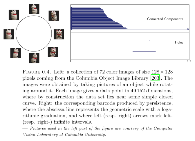
Figure borrowed (thanks in advance Steve) from “Persistence Theory: from Quiver Representations to Data Analysis”
Can we recover that manifold’s structure? Can we understand it with some 2D projection? This would be a great vizualisation.
What about PCA?
Many readers should feel this looks a lot like what Principal Component Analysis (PCA) promesses. Don’t just déjà-vu and change page. While PCA can be useful as a preprocessing step1, PCA plots are often too crowded to insights. Why does PCA look bad?
PCA tries to respect large dissimilarities in the data. Unfortunalty:
- Respecting large scale stucture is irrelevant for data analysis. Far is far, why try to me more specific in what should be a qualitative visualisation?
- Trusting large distances is also tricky in high-dimensional spaces.
- Only small distances are reliable. Objects close in the ambient space may be far away for the manifold’s geodesic distance (think opposite points on a spiral).
- PCA’s cost function means outliers have a large influence. You might need more robust PCA methods.
Because of this, finer details and multi-scale structure are absent from PCA. In addition, PCA only shows proeminent linear projections – and who says the data lies on a linear plane?
In fact, there are many methods that try to respect this local structure (see manifold learning on scikit-learn or this introduction). Among them, tSNE is one of the most effective, successful and insightful.
t-SNE visualization explained
The goal is to represent our data in 2d, such that when 2d points are close together, the data points they represent are actually close together.
As explained elegantly by Andrej Karpathy, we set up two distance metrics in the original and the embedded space and minimize their difference. Those distances are seen as joint-probability distributions. In t-SNE in particular, the original space distance is based on a Gaussian distribution2,
and the embedded space is based on the heavy-tailed Student t-distribution. With a gaussian, far-away points would be seen as too far away in 2d; they would then tend to crush together — the crowding problem:
The KL-divergence formulation [measuring the “difference between the distributions”] has the nice property that it is asymmetric in how it penalizes distances between the two spaces:
- If two points are close in the original space, there is a strong attractive force between the the points in the embedding.
- Conversely, if the two points are far apart in the original space, the algorithm is relatively free to place these points around. Thus, the algorithm preferentially cares about preserving the local structure of the high-dimensional data.
The positions in the lower-dimensionnal space (2d) are optimised by gradient descent.
For more information, watch this presentation by t-SNE’s creator youtube video, or read his clear founding article. Don’t miss his page on t-SNE, with links to the original papers and many implementations.
Does it work?
I’ll let you judge. Here are exemples of outputs for MSNIT digits from the original paper:
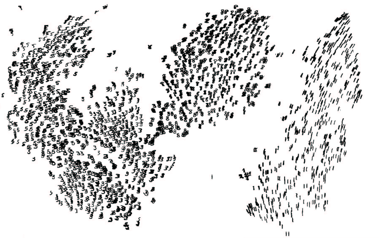 Overall, t-SNE is amazing at revealing structure. Look at the finer details like the slanted eights..!
t-SNE vs PCA is usually one-sided – if you were still wondering. But t-SNE is far from the only manifold-revealing method. For some intuition read Christopher Olah’s post on Visualizing MNIST. You can compare t-SNE vs other manifold learning methods in here.
t-SNE’s performance and complexity
The gradient descent steps express themselves as an n-body problem with attractive and repulsive forces, the later helping separationg points further:
A number of ideas alleviate the naive quadratic gradient descent updates:
- When computing similarities between input points, we only care about non-infinitesimal values, ie neighboorhs of each points. For this we can use a tree-based data structure such as a vantage tree. Finishing this step blocks displaying any “in progress” embedding.
- Using the Barnes-Hut algorithm reduces the complexity of the gradient descent steps to
$O\left(n \log n\right)$in time and$O\left(n\right)$in space — at the cost of approximating. In fact, Barnes-Hut also uses a quad-tree as it tries to summarize contributions of regions. - The origin paper also describes a number of tricks to help convergence…
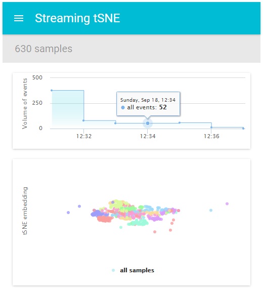
How to use tSNE in streaming scenarios:
Laurens van der Maaten explains why tSNE does not lend itself to streaming so easily:
- t-SNE does not learn a parametrized mapping from the data to R^2.
- Nor does it offer any way to get updates.
Still, he offers some recommendations for those who would like to try:
- Compute tSNE in batch and while waiting train X and Y learners on the previous tSNE mapping.
- Directly learn a mapping, optimizing for tNSE’s loss function, for instance using neural networks.
- Adaptative tSNE, which uses an approximate kNN datastructure that allows insertions and deletions.
In the following posts we will offer implementation details. Stay tuned!
As a bonus, most distances are preserved through even random projects. See sklearn’s page for references of experimental validations. If you strugle PCA’ing your data, try random projections 😄 🍺 🍕 🚀 ↩︎
The variance
$σ_i$is adapted to the local density in the high-dimensional space. t-SNE lets the user specify a “perplexity” parameter that controls the entropy of that local distribution. The entropy amounts to specifying how many neighbours of the current point should have non-small probability values. It works like a continuous choice of k nearest neighboors. ↩︎