Pathfinding algorithms: Road and traffic networks

Maps are among the most used apps on our phones. We always need to go somewhere!

Maps are more complicated than pathfinding

The number of pathfinding-related features available to us via our phones' applications is extraordinary. Making Waze or Uber work requires many expertise domains:

• Collaborative real-time traffic, with traffic prediction, feedback loops and certainly load balancing for the biggest providers.
• Schedule-based transportation networks: for an introduction read this description of Transfer Patterns, or this comparaison versus road networks.
• Time-dependent pathfinding is also crucial in the context of traffic congestion, through mainly quick updates of precomputations or smarter search. Do we want earliest arrival or minimum travel time?
• Multi-modal transportation: cars allow you unlimited travel, but few wants to walk long. This lead to constrained search algorithms involving labels, and optimizing multiple objectives.
• Fleet management for transportation services: you want a vehicule where there is or will be demand. When tranporting multiple passengers, you want to take a route that be fast and fair.
• Detours to points of interest. This might be the basis for ride sharing algorithms. We can also end up into many-to-many pathfinding or delivery problems: traveling salesman, multiple salesmen…
• Alternative itineraries are difficult: k-shortest-paths will give you thousands of tiny variations on the best route… You expect a different route, will only specialized algorithms will yield.

From now on, let’s focus on pathfinding, let’s say the kind used in Google Maps to enable turn-by-turn navigation.

Pathfinding in road networks

Billions of queries surely hit a service like Google Maps daily. People all over the world want to find itineraries across dense and large regions. To cope with the load and answer in a timely manner, using standard graph algorithms like Djikstra’s is not enough. The key is preprocessing. The next sections describe some powerful ideas that allow speed-ups for the “single-source” shortest path problem.

Please forgive omission of key details / inaccuracies; or better: tell me about them!

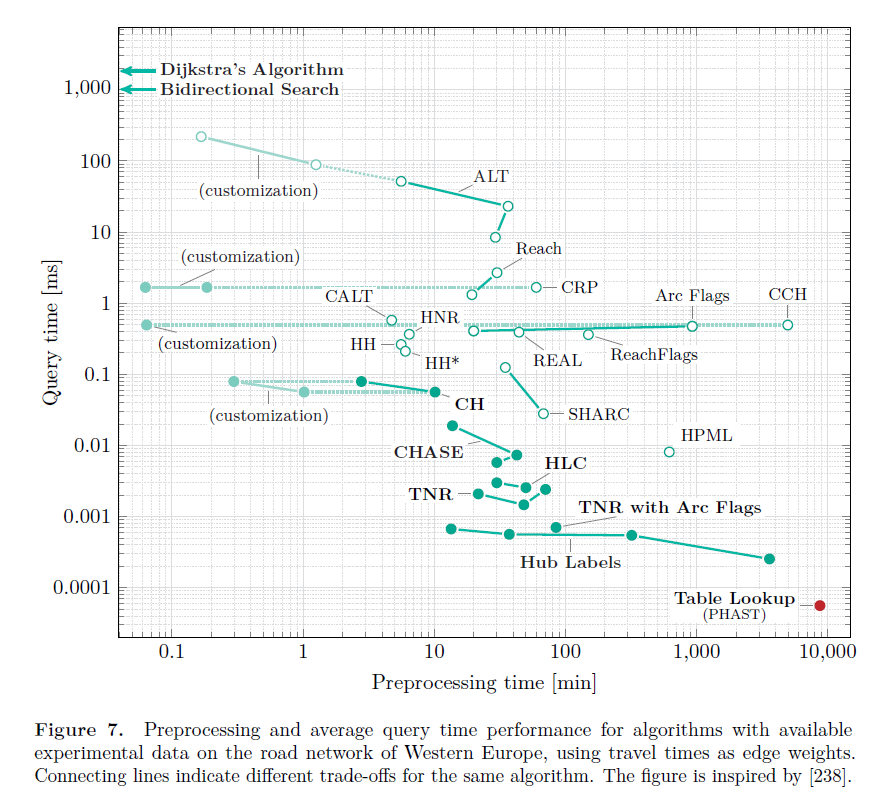
The key goal here is to preprocess reasonnably the network graph so that subsequent queries are sped up as much as possible. Many algorithms exist — leading to enourmous gains over naive Djikstra — with different preprocessing trade-offs:¹

Road networks: the realm of informed search?

A map is not just a graph: it’s embedded in our physical workd. When we go somewhere we usually have an idea of the direction in which we’re heading. The simplest algorithm to use this idea is A*. This improvement over Djikstra adds to the node priority scores a lower-bound estimation of the remaining distance to the target.

However, our goal is usually to minimize travel time – not distance! Finding good travel time bounds is difficult because speed limits vary between roads. The only A* heuristic we could use is “euclidian distance divided by the *maximum* road speed”. In practive it is not that helpful.

Today, no state-of-the-art algorithms make explicit use of map coordinates.

Goal-directed techniques

A* fails in road networks because it uses unrealistic lower bounds. To counter this, we can precompute distances between all pairs of *well-chosen landmarks*², and embed them in our A* heuristic using the triangular inequality. This is the ALT* algorithm.

The distances between landmarks do not give us complete paths. As in many shortcut-based techniques we need to find smart ways to “unpack” the actual shortest path.

In the Geometric Containers approach, all edges store as metadata a hint that lists nodes they lead to via a shortest path. This information is summarized by simple shapes like bounding boxes. This enables aggressively pruning shortest path searches, but at the cost of all-pairs preprocessing (ouch!).

Partitionning road networks

Arc flags improved upon geometric containers by encoding similar information without caring about the geometry. The graph is partitionned into K regions. Then, we find for each edge all regions it can lead to via a shortest path. Usually this information is stored as a K-bit array: arc flags.

Computing all-pairs shortest paths is not necessary: it is enough to look only at paths to regions' boundaries. We could slice regions using a fixed grid, but for best performance the key is to partition the graph using as small frontiers as possible — a hard problem! Subsequent paper introduced improvements such as hierachical regions.

At query time, we need to find out to which region the target belongs. Then (i) outside of the target region we can use the flags to prune all nodes that don’t lead to the target region (ii) within the target region we use Djikstra.

Many ways to exploit graph partitionning

Landmarks and arc flags seem to be a good idea because we “feel” networks can be partitionned into regions by cutting only a few highways. In fact, this property is true for planar graphs; we know road networks are planar except for bridges and tunnels!

A number of Separator Based techniques try use partitions. The key is being able to cut well, while limiting the amount of preprocessing needed to understand shortest paths at the cut boundaries.

Those techniques can involve cutting with either edges or nodes, or hierachies of overlay graphs… See for instance Customizable Route Planning, used by Microsoft, an approach that allows fast re-weighting.

Why road networks lend themselves well to preprocessing

Road networks are more than just planar graphs. When we go somewhere far we know we should first get on the highway. Intuitively, we understand that their hierarchical structure should help pathfinding a lot.

One concept introduced to formalize and justify this idea is a graph’s highway dimension, much similar to the doubling dimension.

Exploiting hierarchy

Highways reach far

We can fasten searches by pruning residential street far from either the source or the destination. This can be implemented by a bi-directional search that considers increasingly high-traffic road. Unfortunately doing this might not always yield correct results and requires tuning. Furthermore, it relies on inflexible labels: what about taking changing traffic conditions into account?

How can we quantify the fact some nodes are more important than others when looking for shortest paths? We expect those nodes have high reach: defined be being in the middle of long shortests paths. This idea led to the REACH algorithm. When doing standard Djikstra searches, nodes with a reach too small to get to the destination are pruned. Computing upper bounds for reach can be done effectively by identifying bounds for nodes of increasingly large reach (using search trees we don’t have to expand far), and removing them from the graph before the next bounds are computed.

As do many algorithms presented here, this approach combines well with other techniques such as A*, landmarks or shortcuts…

Contraction hierachies

We expect to use more important roads in the middle of a shortest path than near the source or target. In the previous section, we mentionned how this can used by a wrong but well-intentioned bi-directional search. Let’s improve upon it and discover³ Contraction Hierarchies, the most efficient common⁴ routing algorithm.

This measure of each arc’s importance could can be quantified by a level. Each bi-directional search should only try to consider increasing levels. The search from the source (resp. target) should explore the upward (resp downward) span of the shortest path. How do we get levels that lead to a correct search?

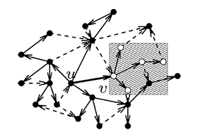
Let’s describe what is a contraction. This operation removes a node while adding necessary⁵ arcs – shortcuts – between its neigboors, so that shortest path distances are preserved. Intuitively, contractions leave a “higher-level” graph. To visualize what a contraction does, look at this figure from Hannah Bast’s Efficient Route Planning course. It helped me a lot!

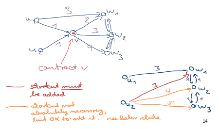
Given a node ordering⁶ describing importance, we now contract all nodes starting by the less important ones. Each step forms new arcs/shortcuts of increasing levels. We stop when we have contracted all nodes. From now on, we compute our bi-directional level-following shortest paths on the graph formed by all nodes and all shortcost at all levels.

“Bounded-hop” techniques

Landmarks understood a powerful idea: having a sense of orientation to “some” nodes is useful. Bounded-hop techniques use a-priori knowledge of intermediary nodes to limit the span of the search.

Transit node routing

To go far away, we tend to always use a small number of nodes: for instance city exits. Transit Node Routing identifies such transit nodes and compute all-pair shortest distances between them. It then assigns to each node the subset of transit nodes (access nodes) that node uses for long shortest paths, along with its distance to them. It is possible to use as little as 5 transit nodes on average. For directed graphs we can have access and exit nodes.

When source and destination nodes are deemed close by a locality filter (geographical distance can do!), a standard shortest path search is used (like for arc flags). When they are deemed far-away, we can find the distance between them by quickly checking possible combinations of source and destination access nodes.

Hub labeling

We could go further with a labeling algorithm, Hub Labeling: rather than storing each node’s local transit nodes (its local hub), we could store all transit nodes⁷ at different scales (its hubs) – up to big continental hubs! – along with the distance to them.

By doing this, we are sure those sets of nodes (aka node labels) obey the cover property: any two nodes have hubs in common in their labels. From there, finding the distance from the source to the destination (plus one hub used) can be found by checking which hub’s usage leads to the shortest path. It is very fast as it basically only involves iterating through two label arrays!

How should be find those hubs? A fairly good candidate is be the set of nodes explore by a Contraction Hierachy search: it makes sense and the cover property comes free. CH are a key ingredient in many advanced algorithms.

Hub labeling can be improved or adapted: many nodes will share the same sequence of large-scale hubs, and it is possible to compress this information.

Graph models for road networks are not always what you would expect

A road network links “nodes” together via road segments you travel on at some expected speed. No surprise: using directed edges will let you model roads better. You might think it is a good idea to compute distances using great circles – but you don’t really need it.

But wait a second, what about getting those turn-by-turn instructions? Well, even before that, how do you model turning restriction? Traffic lights delays? What about your reluctance to turn left, like UPS trucks, or slowdowns from sharp turns?

Shortest path algorithms are all about visiting nodes, but none allows repeated visits, just because we come from an other direction. Navigating around a block to handle a turn restriction seems impossible to handle! Or rather, we should look at (road, turn) couples.

This leads to an alternate representation for our network graph. One where nodes are turns from one intersection to the other, and where edges represente… roads. This is called the edge-expanded model. The graph gets a couple of times bigger, but we gain a lot of flexibility.

MapBox went into some details about this question, take a look! You can also read details on OSRM’s pre-processing flow here. It contains an explanation on how their turn-by-turn guidance and turn-restriction are enabled.

Closing thoughts for network pathfinding

• The amount of work that went into those algorithms is astounding.
• Check PHAST for Djikstra with better performance/locality.
• For extra information, openTripPlanner project has a great bibliography. Reviews of the field are plentiful.
• With all those algorithms, the time to compute a static path is two order of magnitudes lower than the time to retrieve it from a server or plot it..! It might seem overkill, but recall how many extra features we ask of routing engines…!

Stay tuned for the next part of the series…